Summary

Building off of HW 0x02, we are furthering our preparation for our term project by developing a simulation and test a controller for the simplified model of the pivoting platform. Our group decided to attempt both python and matlab to complete this assignment, with the resulting and properly functioning submission to be in matlab, which you will find below. However, you will find our python script linked below as well.

Numerical Parameters

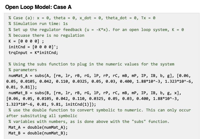
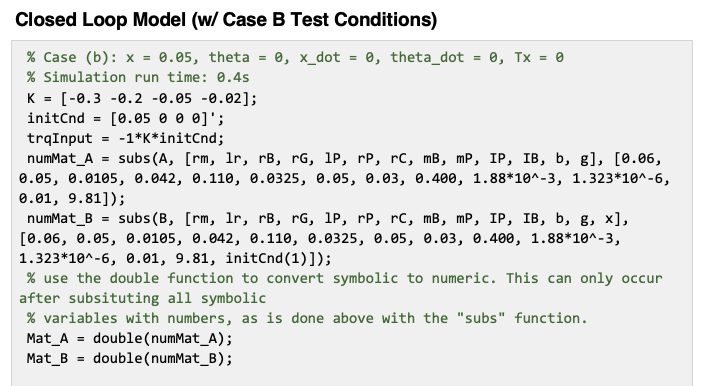
In our simuation, we used the following parameters:

Figure 1. Provided numerical parameters for the simulation

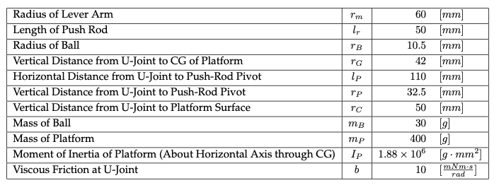
We did not need to design our own controller for this assignment, rather we were given the following gains to test our system performance in closed loop: K = [-0.3, -0.2, -0.05, -0.02] with the units K = [N, N*m, N*s, N*m*s]

Engineering Requirements

• Use the linearization of our system model and express it in state-space form
• Using software, implement model that can be simulated in open-loop given a prescribed set of inital conditions
• Run simulations in open-loop and generate series of plots showing the dynamic response for each state variable
• Simulation A: The ball is initially at rest on a level platform directly above the center of gravity of the platform and there is no torque input from the motor. Run this simulation for 1 [s].
• Simulation B: The ball is initially at rest on a level platform offset horizontally from the center of gravity of the platform by 5 [cm] and there is no torque input from the motor. Run this simulation for 0.4 [s].
• Simulation C: Test simulation in closed-loop by implementing a regulator using full state feedback: u = - Kx and run simulation for at least 20 [s].

Matlab and Simulink Documentation

Matlab Script:

Figure 2. System Parameters Matlab Script

Figure 3. Setting up the Matrices Matlab Script

Figure 4. Plotting Results Matlab Script

Figure 5. Determining the Inverse Matlab Script

Figure 6. Simulation/Case A Open Loop Matlab Script

Figure 7. Simulation/Case B Open Loop Matlab Script

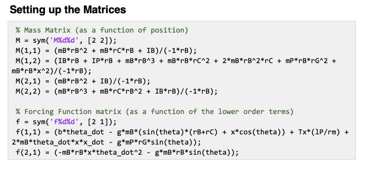
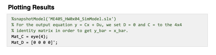
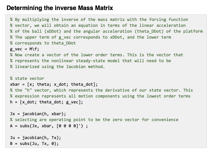
Figure 8. Simulation/Case C Closed Loop using Case B Test Conditions Matlab Script

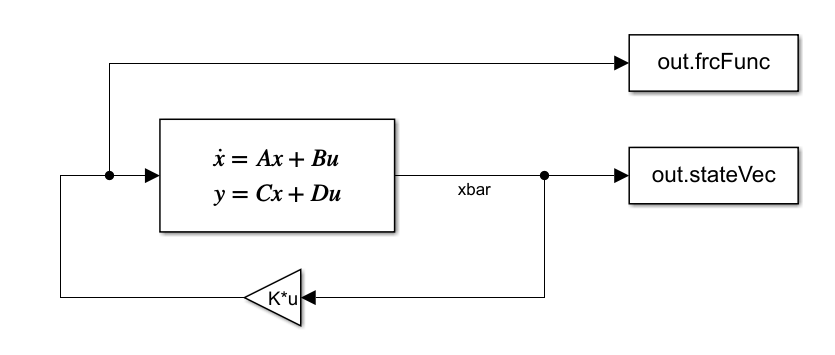
Simulink:

Figure 9. Simulink Model

Simulation Plots

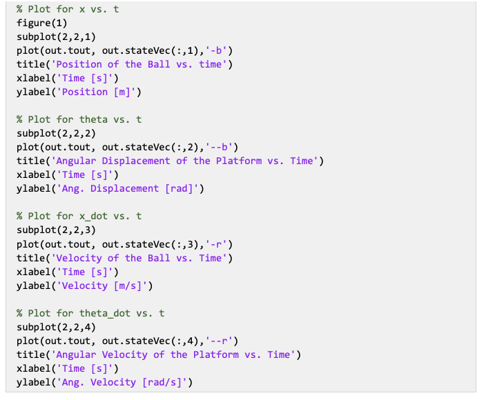
[Simulation A]

Figure 10. Subplots for Simulation/Case A Open Loop

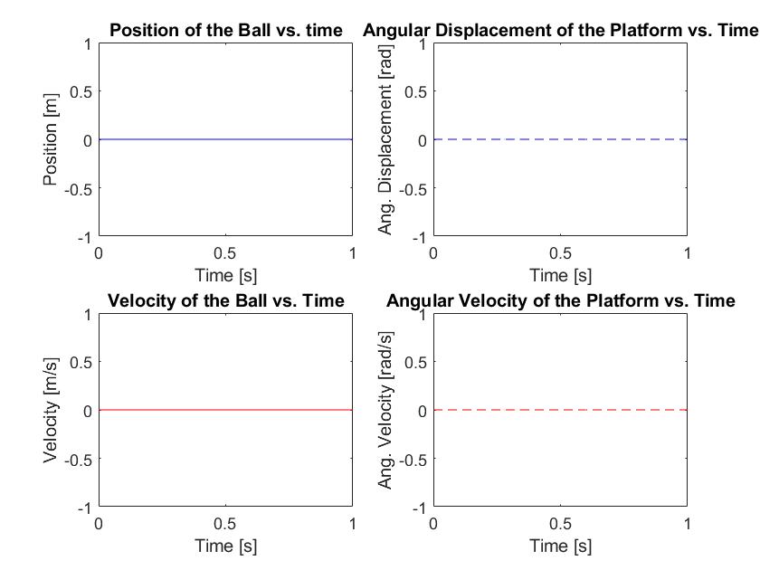
Discussion: The ball is initially placed at the center of the platform, the one stable point in our inherently unstable system. Given that there are no appreciable forces acting on the ball in this simulation, no initial displacements/velocities of the platform or ball, and no torque input from the motor, this system will not deviate from its initial stable point. Therefore, this is a static system, and such behavior is shown by the zero slope lines in all displacement and velocity plots.

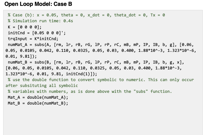
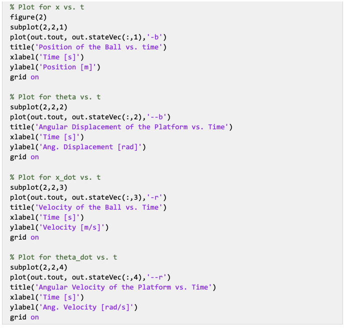
[Simulation B]

Figure 11. Subplots for Simulation/Case B Open Loop

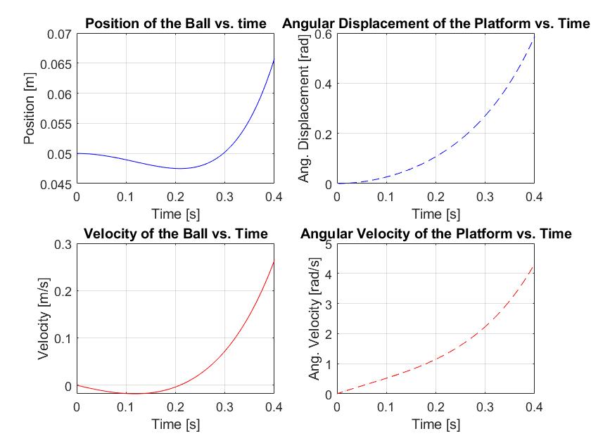
Discussion: The position of the ball as shown in plot [1,1] shows an interesting tendency to climb the incline, moving a direction opposite the tilt. Given that no force is being put into the ball, this tendency is hard to explain. Using newton’s 2nd law it is conceivable that the ball has an small nonzero acceleration as the platform tilts that acts in a direction opposite the motion of the platform. This is confirmed when we look at the velocity graph, whose change with respect to time is distinctly nonlinear and negative, meaning there is a nonzero, negative acceleration in the direction opposite the rotation of the ball. Frictional effects not being appropriately modeled might also have something to do with this physically inconceivable upward motion.

With the oddity explained, the rest of the ball’s position and velocity graph’s show motion we would expect of an open loop controller. The platform will continue to tilt to greater and greater angles [plot[1,2]] at a higher and higher rate [plot [2,2]], increasing towards instability, the point at which the ball falls off the platform.

[Simulation C]

Figure 12. Subplots for Simulation/Case C Closed Loop

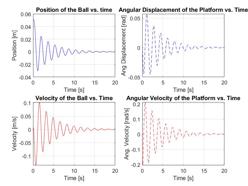
Discussion: As plot[1,1] shows, the ball starts at a position of x = 0.05m, which drives the plate to tilt clockwise about the y-axis, as shown in plot[1, 2]. The system’s regulator detects this initial displacement and attempts to correct the displacement by driving the motor to oppose the ball’s displacement. As a result, even though the platform’s angular velocity starts negative [clockwise] owing to the ball’s initial displacement [plot [2,2]], the clockwise angular velocity slowly decreases as the torque from the motor opposes the ball’s translation and, by association, the clockwise angular displacement of the platform as well. The effect on the ball’s velocity is shown in plot[2,1], where the counteracting torque applied by the motor to the platform drives the ball’s position to change in the direction opposite its initial displacement.

The above description is for one cycle of the closed loop controller. Owing to mechanical losses and the corrective actions of the regulator, the peaks associated with each oscillation will gradually decrease until the ball is more or less returned to a stable state at the center of the platform, which occurs roughly 20 seconds after the initial linear displacement.