Summary

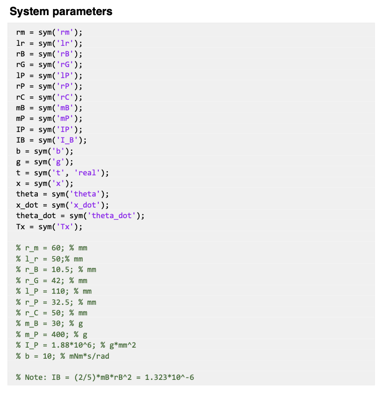
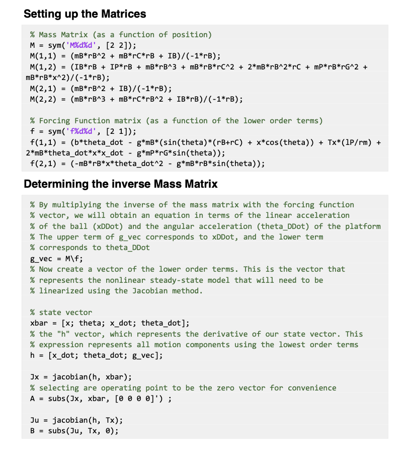
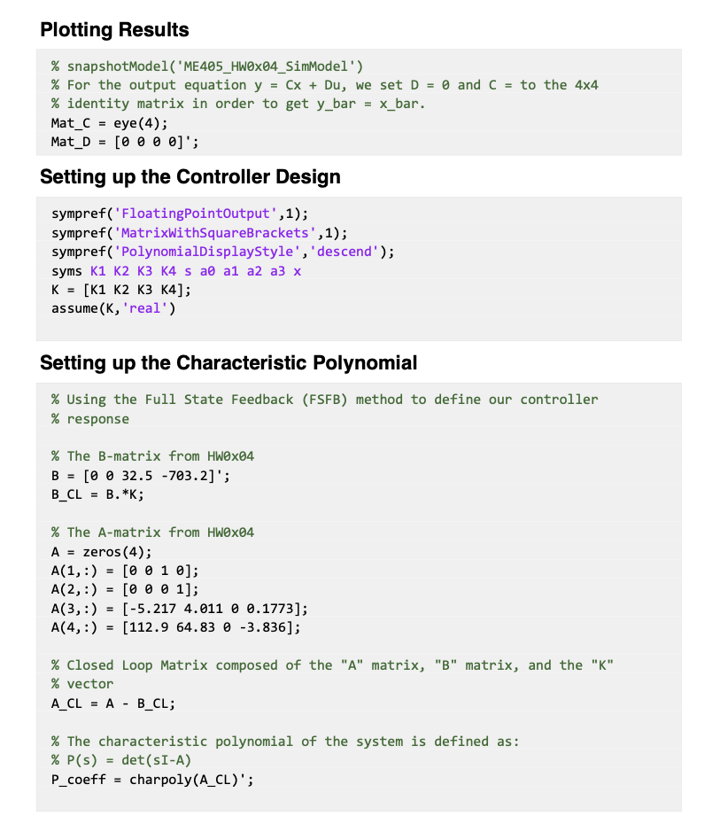
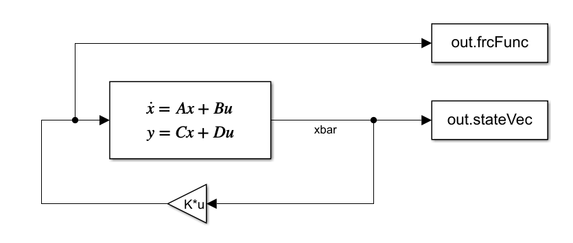
In preparation of our term project and to continue to build off of HW 0x02 and HW 0x04, we developed a closed loop controller for our system model. To ensure consistency and accuracy of our system, we decided to pursue the MatLab/Simulink tools in order to complete our assignment. You will find our Matlab and Simulink documentation below.

Engineering Requirements

• Determine 1x4 gain vector K = [K1, K2, K3, K4]
• Define a method of determining pole locations based criteria
• Find the characteristic polynomial associated with selected pole locations
• Determine the gains K1 through K4.

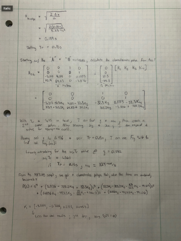
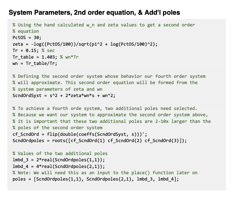
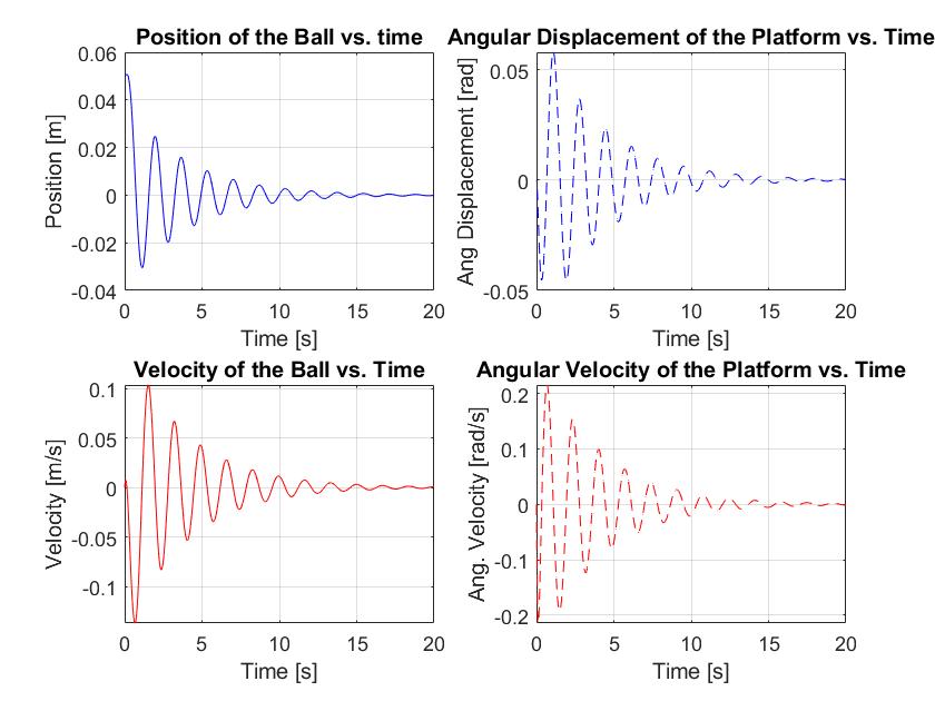
Method of determining pole locations based on criteria was making a dominant pole approximation and choosing two large poles along with two time-domain characteristics like settling time and overshoot percentage.

Hand Calculations

Matlab and Simulink

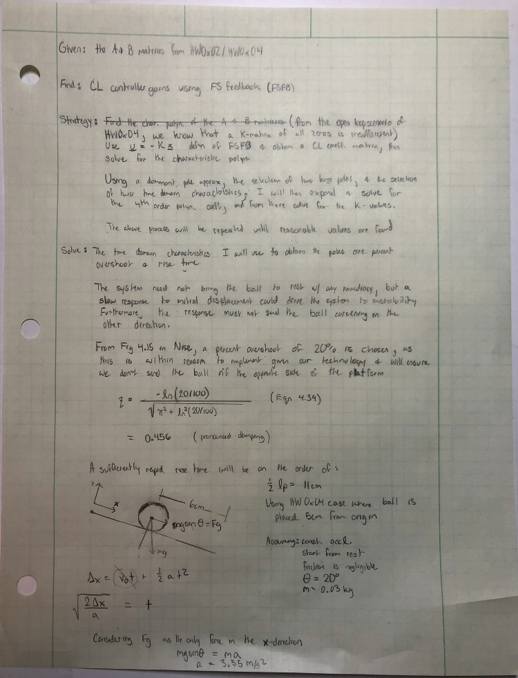
HW 0x05: Developing a Closed Loop Control System for the Balancing Platform

Figure 1. Simulink Model

Results

Verify K values using place() command

Figure 2. Compared calculated results versus results found via place() command

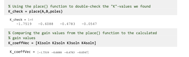
As you can see in Figure 1, the values we outputted matched that of the values resulting from the use of the place() command.

Figure 3. HW 0x04 Controller Plots

Figure 3. HW 0x05 Controller Plots

Discussion & Analysis

1. Show confirmation that your calculated gains correctly place the closed-loop poles at your desired locations

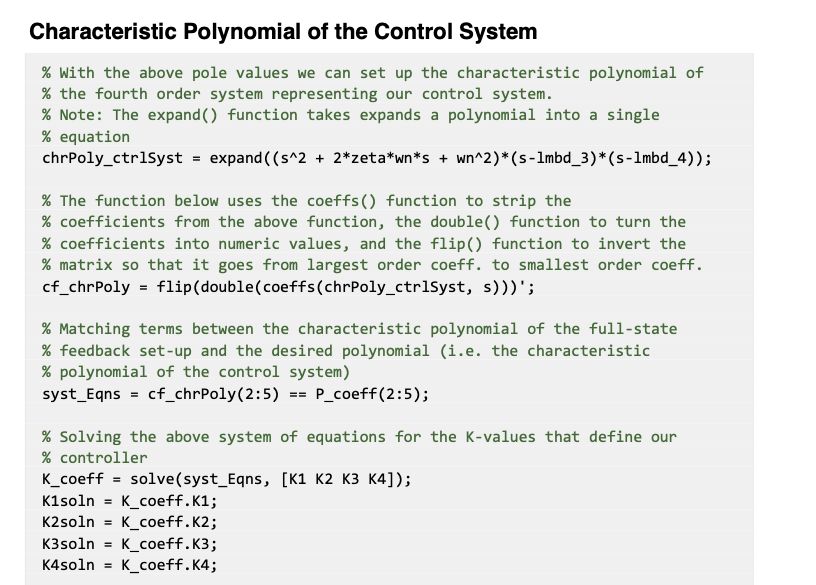
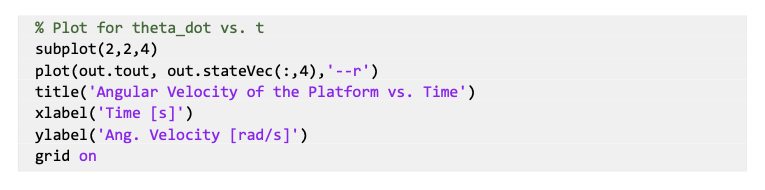
Setting and iterating upon the parameters of rise time and percent overshoot, we arrive at gain values after solving the system characteristic polynomial for the values of "K". When using the place() function to compare the calculated gains